第 7 课补充讲义

算术化是将计算编码为代数约束满足问题的过程。这将检验其正确性的复杂性降低到少量概率代数检查。在证明系统中，算术化的选择会影响IOP的选择范围（见图1）。

图1：证明系统的组成部分。请回顾第5讲（承诺方案）中，承诺方案可用于将交互式预言机证明（IOP）编译成证明系统。

英文原文

Arithmetisation is the encoding of a computation as an algebraic constraint satisfaction problem. This reduces the complexity of verifying its correctness to a few probabilistic algebraic checks. In a proof system, the choice of arithmetisation limits the corresponding range of IOPs that can be used to check it (see Figure 1).

Figure 1: The components of a proof system. Recall from Lecture 3 (Commitment Schemes) that a commitment scheme can be used to compile an interactive oracle proof (IOP) into a proof system.

二次算术程序 (QAPs)

二次算术程序（Quadratic Arithmetic Program，QAP) [9] 是一种将语句转换为多项式上二次方程组的方式。它们可以通过线性交互式证明（LIPs）[10]，代数IOPs [6]，多线性IOPs ([14]，[15]) 进行检验。任何具有乘性复杂度 $n$ 的电路都可以转换为一个 $n$ 次多项式的QAP。

定义1.1. 二次算术程序(QAP)

一个度数为 $d$ 、大小为 $m$ 的二次算术程序 $Q$ 由多项式 ${L_{j} (X)}, {R_{j} (X)}, {O_{j} (X)}, j \in [0, \dots, m - 1]$ 和一个目标多项式 $T (X) := \prod (X - i)_{i = 0}^{d - 1}$ 组成。当赋值 $(1, x_{1}, \dots, x_{m - 1})$ 满足 $Q$ 时，

T (X) ∣ P (X), P (X) := L (X) \cdot R (X) - O (X)

其中 $L (X) := \sum_{j = 0}^{m - 1} x_{j} \cdot L_{j} (X), R (X) := \sum_{j = 0}^{m - 1} x_{j} \cdot R_{j} (X), O (X) := \sum_{j = 0}^{m - 1} x_{j} \cdot O_{j} (X)$ 。

英文原文

The Quadratic Arithmetic Program (QAP) [9] is a way to translate statements into a system of quadratic equations over polynomials. They can be checked by linear interactive proofs (LIPs) [10], algebraic IOPs [6], multilinear IOPs ([14], [15]). Any circuit with multiplicative complexity $n$ can be translated to a QAP over degree- $n$ polynomials.

Definition 1.1. [Quadratic Arithmetic Program (QAP)]

A Quadratic Arithmetic Program Q of degree $d$ and size $m$ consists of polynomials ${L_{j} (X)}, {R_{j} (X)}, {O_{j} (X)}, j \in [0, \dots, m - 1]$ , and a target polynomial $T (X) := \prod (X - i)_{0 = 1}^{d - 1}$ of degree $d$ . An assignment $(1, x_{1}, \dots, x_{m - 1})$ satisfies $Q$ if

T (X) ∣ P (X), P (X) := L (X) \cdot R (X) - O (X)

where $L (X) := \sum_{j = 0}^{m - 1} x_{j} \cdot L_{j} (X), R (X) := \sum_{j = 0}^{m - 1} x_{j} \cdot R_{j} (X), O (X) := \sum_{j = 0}^{m - 1} x_{j} \cdot O_{j} (X)$ .

一阶约束系统 (R1CS)

算术电路可以用简化形式的一阶约束系统(R1CS)表示，而R1CS则可以转换为QAP。

参数系统	算术化	信息理论协议	密码编译器
Groth16 [10]	R1CS	线性交互证明 (LIP)	双线性配对
Marlin [6]	R1CS	代数全息证明 (AHP)	改进的KZG承诺
Spartan [15]	R1CS	变体的sumcheck协议	SPARK
Dory [14]	R1CS	多线性IOP	双线性配对
Nova [13]	放宽的R1CS	多线性IOP	多线性PCS

表1：使用R1CS算术化的证明系统的示例。

在第二讲（Circom 1）中，我们看到了IsZero电路，它检查给定值是否为零的声明。让我们将IsZero转换为一个R1CS电路，然后将其转换为QAP。

template IsZero(){
    signal input in;
    signal output out;

    signal inv;

    inv <−− in != 0 ? 1 / in : 0;

    out <== −in * inv + 1;
    in * out === 0;
}

template IsZero(){
    signal input in;
    signal output out;

    signal inv;

    inv <−− in != 0 ? 1 / in : 0;

    out <== −in * inv + 1;
    in * out === 0;
}

代码1：从comparators.circom中获取的IsZero电路。

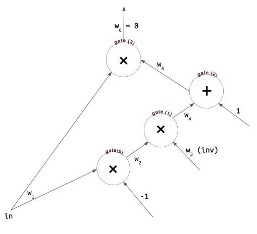
circom的IsZero程序可以“展平”为四个约束条件，每个都采用 左侧 o 右侧 = output 的形式：

\begin{array}{r} w_{1} \cdot (- 1) = w_{2} \\ w_{2} \cdot w_{3} = w_{4} \\ w_{4} + 1 = w_{5} \\ w_{1} \cdot w_{5} = w_{6} \end{array}

在算术电路表示中（左图），每个约束条件对应于一个加法或乘法门。

证明人声称知道一些合法的赋值 $\vec{x} = (x_{1}, x_{2}, x_{3}, x_{4}, x_{5}, x_{6})$ ，使得当将每个值 $a_{i}$ 赋给对应的线路 $w_{i}$ ，并且 $w_{6} = 0$ 时，电路是满足的。对于每个门 $g_{i}$ ，我们创建三个线路向量 $\vec{l_{i}}, {\vec{r}}_{i}, {\vec{o}}_{i}$ ，其中包含门中每个变量 $w_{j}$ 的系数。线路向量还包括一个常数项 $w_{0}$ ：

g_{0} : w_{1} \cdot (- 1) = w_{2} | \begin{array}{r} \begin{array}{cccccccccc} w_{0} & w_{1} & w_{2} & w_{3} & w_{4} & w_{5} & w_{6} \\ {\vec{l}}_{0} = & ( & 0 & 1 & 0 & 0 & 0 & 0 & 0 & ) \\ {\vec{r}}_{0} = & ( & - 1 & 0 & 0 & 0 & 0 & 0 & 0 & ) \\ {\vec{o}}_{0} = & ( & 0 & 0 & 1 & 0 & 0 & 0 & 0 & ) \end{array} \end{array},

g_{1} : w_{2} \cdot w_{3} = w_{4} | \begin{array}{r} \begin{array}{cccccccccc} w_{0} & w_{1} & w_{2} & w_{3} & w_{4} & w_{5} & w_{6} \\ {\vec{l}}_{1} = & ( & 0 & 0 & 1 & 0 & 0 & 0 & 0 & ) \\ {\vec{r}}_{1} = & ( & 0 & 0 & 0 & 1 & 0 & 0 & 0 & ) \\ {\vec{o}}_{1} = & ( & 0 & 0 & 0 & 0 & 1 & 0 & 0 & ) \end{array} \end{array},

\begin{array}{r} g_{2} : w_{4} + 1 = w_{5} \\ (w_{4} + 1) \cdot 1 = w_{5} \end{array} | \begin{array}{r} \begin{array}{cccccccccc} w_{0} & w_{1} & w_{2} & w_{3} & w_{4} & w_{5} & w_{6} \\ {\vec{l}}_{2} = & ( & 1 & 0 & 0 & 0 & 1 & 0 & 0 & ) \\ {\vec{r}}_{2} = & ( & 1 & 0 & 0 & 0 & 0 & 0 & 0 & ) \\ {\vec{o}}_{2} = & ( & 0 & 0 & 0 & 0 & 0 & 1 & 0 & ) \end{array} \end{array},

g_{3} : w_{1} \cdot w_{5} = w_{6} | \begin{array}{r} \begin{array}{cccccccccc} w_{0} & w_{1} & w_{2} & w_{3} & w_{4} & w_{5} & w_{6} \\ {\vec{l}}_{3} = & ( & 0 & 1 & 0 & 0 & 0 & 0 & 0 & ) \\ {\vec{r}}_{3} = & ( & 0 & 0 & 0 & 0 & 0 & 1 & 0 & ) \\ {\vec{o}}_{3} = & ( & 0 & 0 & 0 & 0 & 0 & 0 & 1 & ) \end{array} \end{array} .

现在，我们将每个左边的 $l_{i}$ 线向量收集到矩阵 $L = (\vec{l_{0}}, \vec{l_{1}}, \vec{l_{2}}, \vec{l_{3}})$ 中，对于右边的 $\vec{r_{i}}$ 线向量同样如此，而输出 $\vec{o_{i}}$ 向量也是如此： $R = (\vec{r_{0}}, \vec{r_{1}}, \vec{r_{2}}, \vec{r_{3}})$ ， $O = (\vec{o_{0}}, \vec{o_{1}}, \vec{o_{2}}, \vec{o_{3}})$ 。

\begin{aligned} L = \begin{array}{cc} \begin{array}{cc} \begin{array}{ccccccc} w_{0} & w_{1} & w_{2} & w_{3} & w_{4} & w_{5} & w_{6} \end{array} \\ (\begin{array}{ccccccc} 0 & 1 & 0 & 0 & 0 & 0 & 0 \\ 0 & 0 & 1 & 0 & 0 & 0 & 0 \\ 1 & 0 & 0 & 0 & 1 & 0 & 0 \\ 0 & 1 & 0 & 0 & 0 & 0 & 0 \end{array}) & \begin{array}{l} {\vec{l}}_{0} \\ {\vec{l}}_{1} \\ {\vec{l}}_{2} \\ {\vec{l}}_{3} \end{array} \end{array} \end{array}, \end{aligned}

\begin{aligned} R = \begin{array}{cc} \begin{array}{cc} \begin{array}{ccccccc} w_{0} & w_{1} & w_{2} & w_{3} & w_{4} & w_{5} & w_{6} \end{array} \\ (\begin{array}{ccccccc} - 1 & 0 & 0 & 0 & 0 & 0 & 0 \\ 0 & 0 & 0 & 1 & 0 & 0 & 0 \\ 1 & 0 & 0 & 0 & 0 & 0 & 0 \\ 0 & 0 & 0 & 0 & 0 & 1 & 0 \end{array}) & \begin{array}{l} {\vec{r}}_{0} \\ {\vec{r}}_{1} \\ {\vec{r}}_{2} \\ {\vec{r}}_{3} \end{array} \end{array} \end{array}, \end{aligned}

\begin{aligned} O = \begin{array}{cc} \begin{array}{cc} \begin{array}{ccccccc} w_{0} & w_{1} & w_{2} & w_{3} & w_{4} & w_{5} & w_{6} \end{array} \\ (\begin{array}{ccccccc} 0 & 0 & 1 & 0 & 0 & 0 & 0 \\ 0 & 0 & 0 & 0 & 1 & 0 & 0 \\ 0 & 0 & 0 & 0 & 0 & 1 & 0 \\ 0 & 0 & 0 & 0 & 0 & 0 & 1 \end{array}) & \begin{array}{l} {\vec{o}}_{0} \\ {\vec{o}}_{1} \\ {\vec{o}}_{2} \\ {\vec{o}}_{3} \end{array} \end{array} \end{array} . \end{aligned}

矩阵 $L, R, O$ 和见证向量 $\vec{x} = (1, x_{1}, x_{2}, x_{3}, x_{4}, x_{5}, x_{6})$ 一起构成了IsZero电路的R1CS形式。满足条件的向量 $\vec{x}$ 可以实现方程 $L \cdot \vec{x} + R \cdot \vec{x} - O \cdot \vec{x} = 0$ 。

英文原文

Arithmetic circuits can be expressed a simplified form known as Rank-1 Constraint System (R1CS), which can in turn be transformed into a QAP.

Argument system	Arithmetization	Information-theoretic protocol	Cryptographic compiler
Groth16 [10]	R1CS	linear interactive proof (LIP)	bilinear pairings
Marlin [6]	R1CS	algebraic holographic proof (AHP)	adapted KZG commitment
Spartan [15]	R1CS	variant of sumcheck protocol	SPARK
Dory [14]	R1CS	multilinear IOP	bilinear pairings
Nova [13]	Relaxed R1CS	multilinear IOP	multilinear PCS

Table 1: Examples of proof systems which make use of R1CS arithmetisation.

In Lecture 2 (Circom 1), we saw the Is Zero circuit, which checks a claim about whether a given value is zero. Let's convert Is eero into an R1CS circuit, and then transform it into a QAP.

template IsZero(){
    signal input in;
    signal output out;

    signal inv;

    inv <−− in != 0 ? 1 / in : 0;

    out <== −in * inv + 1;
    in * out === 0;
}

template IsZero(){
    signal input in;
    signal output out;

    signal inv;

    inv <−− in != 0 ? 1 / in : 0;

    out <== −in * inv + 1;
    in * out === 0;
}

Listing 1: The Iszero circuit, taken from comparators. circom in circomlib.

The circom Iszero program can be "flattened" into four constraints, each of the form left o right = output:

\begin{array}{r} w_{1} \cdot (- 1) = w_{2} \\ w_{2} \cdot w_{3} = w_{4} \\ w_{4} + 1 = w_{5} \\ w_{1} \cdot w_{5} = w_{6} \end{array}

In the arithmetic circuit representation (left), each of these constraints corresponds to an addition or multiplication gate.

The prover is claiming to know some legal assignment $\vec{x} = (x_{1}, x_{2}, x_{3}, x_{4}, x_{5}, x_{6})$ , so that when each value $a_{i}$ is assigned to corresponding wire $w_{i}$ , and $w_{6} = 0$ , the circuit is satisfied. For each gate $g_{i}$ , we create three wire vectors $\vec{l_{i}}, {\vec{r}}_{i}, {\vec{o}}_{i}$ , containing the coefficients of each variable $w_{j}$ at the gate. The wire vectors also include a constant term $w_{0}$ :

g_{0} : w_{1} \cdot (- 1) = w_{2} | \begin{array}{r} \begin{array}{cccccccccc} w_{0} & w_{1} & w_{2} & w_{3} & w_{4} & w_{5} & w_{6} \\ {\vec{l}}_{0} = & ( & 0 & 1 & 0 & 0 & 0 & 0 & 0 & ) \\ {\vec{r}}_{0} = & ( & - 1 & 0 & 0 & 0 & 0 & 0 & 0 & ) \\ {\vec{o}}_{0} = & ( & 0 & 0 & 1 & 0 & 0 & 0 & 0 & ) \end{array} \end{array},

g_{1} : w_{2} \cdot w_{3} = w_{4} | \begin{array}{r} \begin{array}{cccccccccc} w_{0} & w_{1} & w_{2} & w_{3} & w_{4} & w_{5} & w_{6} \\ {\vec{l}}_{1} = & ( & 0 & 0 & 1 & 0 & 0 & 0 & 0 & ) \\ {\vec{r}}_{1} = & ( & 0 & 0 & 0 & 1 & 0 & 0 & 0 & ) \\ {\vec{o}}_{1} = & ( & 0 & 0 & 0 & 0 & 1 & 0 & 0 & ) \end{array} \end{array},

\begin{array}{r} g_{2} : w_{4} + 1 = w_{5} \\ (w_{4} + 1) \cdot 1 = w_{5} \end{array} | \begin{array}{r} \begin{array}{cccccccccc} w_{0} & w_{1} & w_{2} & w_{3} & w_{4} & w_{5} & w_{6} \\ {\vec{l}}_{2} = & ( & 1 & 0 & 0 & 0 & 1 & 0 & 0 & ) \\ {\vec{r}}_{2} = & ( & 1 & 0 & 0 & 0 & 0 & 0 & 0 & ) \\ {\vec{o}}_{2} = & ( & 0 & 0 & 0 & 0 & 0 & 1 & 0 & ) \end{array} \end{array},

g_{3} : w_{1} \cdot w_{5} = w_{6} | \begin{array}{r} \begin{array}{cccccccccc} w_{0} & w_{1} & w_{2} & w_{3} & w_{4} & w_{5} & w_{6} \\ {\vec{l}}_{3} = & ( & 0 & 1 & 0 & 0 & 0 & 0 & 0 & ) \\ {\vec{r}}_{3} = & ( & 0 & 0 & 0 & 0 & 0 & 1 & 0 & ) \\ {\vec{o}}_{3} = & ( & 0 & 0 & 0 & 0 & 0 & 0 & 1 & ) \end{array} \end{array},

Now, we collect each of the left $l_{i}$ wire vectors into a matrix $L = (\vec{l_{0}}, \vec{l_{1}}, \vec{l_{2}}, \vec{l_{3}})$ , and likewise for the right $R = ({\vec{r}}_{0}, {\vec{r}}_{1}, {\vec{r}}_{2}, {\vec{r}}_{3})$ and output $O = ({\vec{o}}_{0}, {\vec{o}}_{1}, {\vec{o}}_{2}, {\vec{o}}_{3})$ vectors:

\begin{aligned} L = \begin{array}{cc} \begin{array}{cc} \begin{array}{ccccccc} w_{0} & w_{1} & w_{2} & w_{3} & w_{4} & w_{5} & w_{6} \end{array} \\ (\begin{array}{ccccccc} 0 & 1 & 0 & 0 & 0 & 0 & 0 \\ 0 & 0 & 1 & 0 & 0 & 0 & 0 \\ 1 & 0 & 0 & 0 & 1 & 0 & 0 \\ 0 & 1 & 0 & 0 & 0 & 0 & 0 \end{array}) & \begin{array}{l} {\vec{l}}_{0} \\ {\vec{l}}_{1} \\ {\vec{l}}_{2} \\ {\vec{l}}_{3} \end{array} \end{array} \end{array}, \end{aligned}

\begin{aligned} R = \begin{array}{cc} \begin{array}{cc} \begin{array}{ccccccc} w_{0} & w_{1} & w_{2} & w_{3} & w_{4} & w_{5} & w_{6} \end{array} \\ (\begin{array}{ccccccc} - 1 & 0 & 0 & 0 & 0 & 0 & 0 \\ 0 & 0 & 0 & 1 & 0 & 0 & 0 \\ 1 & 0 & 0 & 0 & 0 & 0 & 0 \\ 0 & 0 & 0 & 0 & 0 & 1 & 0 \end{array}) & \begin{array}{l} {\vec{r}}_{0} \\ {\vec{r}}_{1} \\ {\vec{r}}_{2} \\ {\vec{r}}_{3} \end{array} \end{array} \end{array}, \end{aligned}

\begin{aligned} O = \begin{array}{cc} \begin{array}{cc} \begin{array}{ccccccc} w_{0} & w_{1} & w_{2} & w_{3} & w_{4} & w_{5} & w_{6} \end{array} \\ (\begin{array}{ccccccc} 0 & 0 & 1 & 0 & 0 & 0 & 0 \\ 0 & 0 & 0 & 0 & 1 & 0 & 0 \\ 0 & 0 & 0 & 0 & 0 & 1 & 0 \\ 0 & 0 & 0 & 0 & 0 & 0 & 1 \end{array}) & \begin{array}{l} {\vec{o}}_{0} \\ {\vec{o}}_{1} \\ {\vec{o}}_{2} \\ {\vec{o}}_{3} \end{array} \end{array} \end{array} . \end{aligned}

The $L, R, O$ matrices, along with our witness vector $\vec{x} = (1, x_{1}, x_{2}, x_{3}, x_{4}, x_{5}, x_{6})$ , gives the

第 7 课 补充讲义 ​

二次算术程序 (QAPs) ​

一阶约束系统 (R1CS) ​

第 7 课补充讲义

二次算术程序 (QAPs)

一阶约束系统 (R1CS)